Thursday, December 11, 2014

Mixed Signals and Monetary Policy Discretion

Two recent Economic Letters from the Federal Reserve Bank of San Francisco highlight the difficulty of making monetary policy decisions when alternative measures of labor market slack and the output gap give mixed signals. In Monetary Policy when the Spyglass is Smudged, Early Elias, Helen Irvin, and Òscar Jordà show that conventional policy rules based on the output gap and on the deviation of the unemployment rate from its natural rate generate wide-ranging policy rate prescriptions. Similarly, in Mixed Signals: Labor Markets and Monetary Policy, Canyon Bosler, Mary Daly, and Fernanda Nechio calculate the policy rate prescribed by a Taylor rule under alternative measures of labor market slack. The figure below illustrates the large divergence in alternative prescribed policy rates since the Great Recession.

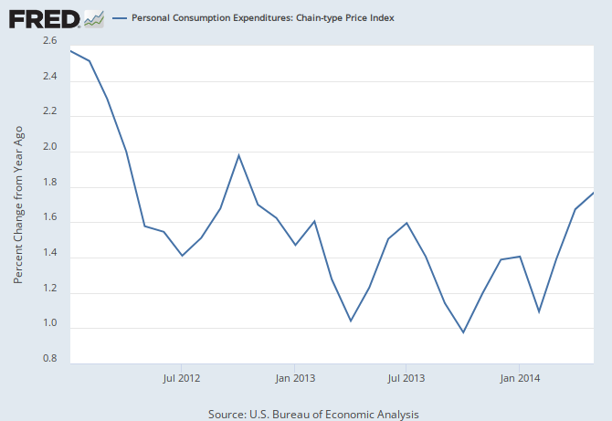
Source: Bosler, Daly, and Nechio (2014), Figure 2
Uncertainty about the state of the labor market makes monetary policy more challenging and requires more discretion and judgment on the part of policymakers. What does discretion and judgment look like in practice? I think it should involve reasoning qualitatively to determine if some decisions lead to possible outcomes that are definitively worse than others. For example, here's how I would reason through the decision about whether to raise the policy rate under high uncertainty about the labor market:

Suppose it is May and the Fed is deciding whether to increase the target rate by 25 basis points. Assume inflation is still at or slightly below 2%, and the Fed would like to tighten monetary policy if and only if the "true" state of the labor market x is sufficiently high, say above some threshold X. The Fed does not observe x but has some very noisy signals about it.  They think there is about a fifty-fifty chance that x is above X, so it is not at all obvious whether tightening is appropriate. There are four possible scenarios:

  1. The Fed does not increase the target rate, and it turns out that x>X.
  2. The Fed does not increase the target rate, and it turns out that x<X.
  3. The Fed does increase the target rate, and it turns out that x>X.
  4. The Fed does increase the target rate, and it turns out that x>X.

Cases (2) and (3) are great. In case (2), the Fed did not tighten when tightening was not appropriate, and in case (3), the Fed tightened when tightening was appropriate. Cases (1) and (4) are "mistakes." In case (1), the Fed should have tightened but did not, and in case (4), the Fed should not have tightened but did. Which is worse?

If we think just about immediate or short-run impacts, case (1) might mean inflation goes higher than the Fed wants and x goes even higher above X; case (4) might mean unemployment goes higher than the Fed wants and x falls even further below X. Maybe you have an opinion on which of those short-run outcomes is worse, or maybe not. But the bigger difference between the outcomes comes when you think about the Fed's options at its subsequent meeting. In case (1), the Fed could choose how much they want to raise rates to restrain inflation. In case (4), the Fed could keep rates constant or reverse the previous meeting's rate increase.

In case (4), neither option is good. Keeping the target at 25 basis points is too restrictive. Labor market conditions were bad to begin with and keeping policy tight will make them worse. But reversing the rate increase is a non-starter. The markets expect that after the first rate increase, rates will continue on an upward trend, as in previous tightening episodes. Reversing the rate increase would cause financial market turmoil, damage credibility, and require policymakers to admit that they were wrong. Case (1) is much more attractive. I think any concern that inflation could take off and get out of control is unwarranted. In the space between two FOMC meetings, even if inflation were to rise above target, inflation expectations are not likely to rise too far. The Fed could easily restrain expectations at the next meeting by raising rates as aggressively as needed.

So going back to the four possible scenarios, (2) and (3) are good, and (4) is much worse than (1). If the Fed raises rates, scenarios (3) and (4) are about equally likely. If the Fed holds rates constant, (1) and (2) are about equally likely. Thus, holding rates constant under high uncertainty about the state of the labor market is a better option than potentially raising rates too soon.

Sunday, December 7, 2014

Most Households Expect Interest Rates to Increase by May

Two new posts on the New York Federal Reserve's Liberty Street Economics Blog describe methods of inferring interest rate expectations from interest rate futures and forwards and from surveys conducted by the Trading Desk of the New York Fed. In a post at the Atlanta Fed's macroblog, "Does Forward Guidance Reach Main Street?," economists Mike BryanBrent Meyer, and Nicholas Parker, ask, "But what do we know about Main Street’s perspective on the fed funds rate? Do they even have an opinion on the subject?"

To broach this question, they use a special question on the Business Inflation Expectations (BIE) Survey. A panel of businesses in the Sixth District were asked to assign probabilities that the federal funds rate at the end of 2015 would fall into various ranges. The figure below compares the business survey responses to the FOMC's June projection. The similarity between businesspeoples' expectations and FOMC members' expectations for the fed funds rate is taken as an indication that forward guidance on the funds rate has reached Main Street.


What about the rest of Main Street-- the non-business-owners? We don't know too much about forward guidance and the average household. I looked at the Michigan Survey of Consumers for some indication of households' interest rate expectations. One year ago, in December 2013, 61% of respondents on the Michigan Survey said they expected interest rates to rise in the next twelve months. Only a third of consumers expected rates to stay approximately the same. According to the most recently-available edition of the survey, from May 2014, 63% of consumers expect rates to rise by May 2015.

The figure below shows the percent of consumers expecting interest rates to increase in the next twelve months in each survey since 2008. I use vertical lines to indicate several key dates. In December 2008, the federal funds rate target was reduced to 0 to 0.25%, marking the start of the zero lower bound period. Nearly half of consumers in 2009 and 2010 expected rates to rise over the next year. In August 2011, Fed officials began using calendar-based forward guidance when they announced that they would keep rates near zero until at least mid-2013. Date-based forward guidance continued until December 2012. Over this period, less than 40% of consumers expected rate increases.

In December 2012, the Fed adopted the Evans Rule, announcing that the fed funds rate would remain near zero until the unemployment rate fell to 6.5%. In December 2013, the Fed announced a modest reduction in the pace of its asset purchases, emphasizing that this "tapering" did not indicate imminent rate increases. The share of consumers expecting rate increases made a large jump from 55% in June 2013 to 68% in July 2013, and has remained in the high-50s to mid-60s since then.


But since 1978, the percent of consumers expecting an increase in interest rates has tracked reasonably closely with the realized change in the federal funds rate over the next twelve months (fed funds rate in month t+12 minus fed funds rate in month t). In the figure below, the correlation coefficient is 0.26. As a back-of-the-envelop calculation, if we regress the change in the federal funds rate in twelve months on the percent of consumers expecting a rate increase, the regression coefficients indicate that when 63% of consumers expect a rate increase, that predicts a 25 basis points rise in rates in the next year.


This survey data does not tell us for sure that forward guidance has reached Main Street. The survey does not specifically refer to the federal funds rate, just to interest rates in general. And households could simply have noticed that rates have been low for a long time and expect them to increase, even without hearing the Fed's forward guidance.  In an average month, 51% of consumers expect rates to rise over the next year, with a standard deviation of 15%. So the values we're seeing lately are about a standard deviation above the historical average, but they have been higher historically. In the third and fourth quarters of 1994, after the Fed had already begun tightening interest rates, 75-80% of consumers expected further rate increases. At the start of 1994, however, only half of consumers anticipated the rate increases that would come.

In May 2004, the FOMC noted that accommodation could “be removed at a pace that is likely to be measured.” That month, 85% of consumers (a historical maximum) correctly expected rates to increase.

Monday, December 1, 2014

A Cyber Monday Message of Thanks

Cyber Monday may just be a marketing tool, but I'll take it as an opportunity to send a cyber-message of thanksgiving out to all of you who are connected to me through my blog.

I started this blog in September 2012 but only started posting regularly in January 2013, after attending a panel discussion at the 2013 AEA meetings called "Models or Muddles: How the Press Covers Economics and the Economy." The panel members, Tyler Cowen, Adam Davidson, Kelly Evans, Chrystia Freeland, and David Wessel, discussed the importance and challenge of writing intellectually upright and emotionally compelling economic journalism. I took their discussion as an invitation to try my hand at economics blogging, and I immensely appreciate every one of you who have read, shared, criticized, complemented, and challenged my writing along the way. Most of you are anonymous, but several of you I feel that I know personally. All of you have helped me improve and inspired me to continue.

I blog mostly for myself. It is a remarkable opportunity to think through new ideas, evaluate recent research, and learn about important policy issues. When I started the blog, I was quite new to economics. I was a math major as an undergraduate, so my first year of graduate school at Berkeley was a boot camp-style introduction to economic theory and analysis. Now, in my final year of graduate school, I am still relatively new to the field, but blogging has helped me develop a broader and more nuanced and contextualized understanding of economics than I could have achieved from school alone.

I blog mostly for myself, but not only for myself. I entered an economics Ph.D. program because I fundamentally wanted to help people and make a difference in the world, as naive as that may sound. Now, looking over at my brand new baby daughter, that is still what I want, even more so than five years ago, though I think I have a more subtle understanding of "making a difference" than I used to. That is also why I want to thank you, readers. I do not give you investment advice, teach you how to get rich quick, or provide juicy ad hominem attacks to entertain you. If you're reading my blog, it's probably because you also have an intellectual interest in economics also stemming, I like to believe, from your desire for a better world. Thanks.

Tuesday, November 25, 2014

Regime Change From Roosevelt to Rousseff

I've written another post for the Berkeley Center for Latin American Studies blog:
President Franklin Delano Roosevelt was elected in October 1932, in the midst of the Great Depression. High unemployment, severely depressed spending, and double-digit deflation plagued the economy. Shortly after his inauguration in March 1933, a dramatic turnaround occurred. Positive inflation was restored, and 1933 to 1937 was the fastest four-year period of output growth in peacetime in United States history. 
How did such a transformation occur? Economists Peter Temin and Barrie Wigmore attribute the recovery to a “regime change.” In the economics literature, regime change refers to the idea that a set of new policies can have major effects by rapidly and sharply changing expectations. A regime change can occur when a policymaker credibly commits to a new set of policies and goals.... 
In short, Roosevelt stated and proved that he was willing to do whatever it would take to end deflation and restore economic growth. As Roosevelt proclaimed on October 22, 1933: “If we cannot do this one way, we will do it another. Do it, we will.” 
Almost all politicians promise change but few manage such drastic transformation. In Brazil’s closely contested presidential election this October, incumbent President Dilma Rousseff won reelection with a three-point margin over centrist candidate Aecio Neves. Rouseff told supporters, “I know that I am being sent back to the presidency to make the big changes that Brazilian society demands. I want to be a much better president than I have been until now.” 
Rousseff’s rhetoric of “big changes” refers in large part to the Brazilian economy, which is plagued with stagnant growth, high inflation, and a strained federal budget. Brazil’s currency, the real, hit a nine-year low following Rousseff’s victory, and the stock market also tumbled. This market tumult reflects investors’ doubts about the Rousseff administration’s intention and ability to enact effective reforms. Investors viewed Neves as the pro-business, anti-interventionist candidate and are unconvinced that Rousseff will act decisively to restore fiscal discipline and rein in inflation. In other words, Rousseff’s talk of change is not fully credible in the way that Roosevelt’s was... 
Though Rousseff is taking some actions to improve business conditions, restore fiscal discipline, and reduce inflation, the problem is that they are being enacted quietly and reluctantly rather than being trumpeted as part of a broader vision of reform. The key to regime change is that the effects of policy changes depend crucially on how the changes are presented and perceived. Economic policies work not only through direct channels but also through signaling and expectations. For example, a small rise in fuel prices and a reduction in state bank subsidized lending may have small direct effects, but if they are viewed as signals that the president is wholeheartedly embracing market-friendly reforms, the effects will be much greater. So far, despite Rousseff’s campaign slogan — “new government, new ideas” — she hasn’t credibly committed to a new regime.
Read the complete article and my pre-election Brazil article at the CLAS blog.

Monday, November 10, 2014

Reading Keynes at the Zero Lower Bound

The developed economies of Japan, the United States, and the Eurozone are currently experiencing very low short-term rates, so low that they are considered to be at the “zero lower bound” of possibility. This effectively paralyzes conventional monetary policy. As a consequence, monetary authorities have turned to unconventional and controversial policies such as “Quantitative Easing,” “Maturity Extension,” and “Low for Long Forward Guidance.” John Maynard Keynes in The General Theory offered a rich analysis of the problems that appear at the zero lower bound and advocated the very same unconventional policies that are now being pursued. Keynes’s comments on these issues are rarely mentioned in the current discussions because the subsequent simplifications and the bowdlerization of his model obliterated this detail. It was only later that his characterization of a lower bound to interest rates would be dubbed a “Liquidity Trap.” This essay employs Keynes’s analysis to retell the economic history of the Great Depression in the United States. Keynes’s rationale for unconventional policies and his expectations of their effect remain surprisingly relevant today. I suggest that in both the Depression and the Great Recession the primary impact on interest rates was produced by lowering expectations about the future path of rates rather than by changing the risk premiums that attach to yields of different maturities. The long sustained period when short term rates were at the lower bound convinced investors that rates were likely to remain near zero for several more years. In both cases the treatment proved to be very slow to produce a significant response, requiring a sustained zero-rate policy for four years or longer.
Sutch notes that "the General Theory is a notoriously unreadable book, one that required others to interpret and popularize its message." Since Keynes did not use the phrase "liquidity trap"--it was coined by Dennis Robertson in 1940--interpreting Keynes' policy prescriptions in a liquidity trap is contentious. Sutch reinterprets the theory of the liquidity trap from the General Theory, then examines the impact of Federal Reserve and Treasury policies during the Great Depression in light of his interpretation.

Sutch outlines Keynes' three theoretical reasons why an effective floor to long-term interest rates might be encountered at the depth of a depression:
(1) Since the term structure of interest rates will rise with maturity when short-term rates are low, a point might be reached where continued open-market purchases of shortterm government debt would reduce the short-term rate to zero before producing a sufficient decline in the risk-free long-term rate [Keynes 1936: 201-204 and 233]. 
(2) It is, at least theoretically, possible that the demand for money (called “liquidity preference” by Keynes) could become “virtually absolute” at a sufficiently low longterm interest rate and, if so, then increases in the money supply would be absorbed completely by hoarding [Keynes 1936: 172 and 207-208]. 
(3) The default premiums included as a portion of the interest charged on business loans and on the return to corporate securities could become so great that it would prove impossible to bring down the long-term rate of interest relevant for business decisions even though the risk-free long-term rate was being reduced by monetary policy [Keynes 1936: 144-145].
The first two reasons, Sutch notes, are often conflated  because of a tendency in the post-Keynesian literature to drop short-term assets from the model. The third reason, called "lender's risk," is typically neglected in textbooks and empirical studies.

In Keynes' view, the Great Depression was triggered by a collapse in investment in 1929, prior to the Wall Street crash in the fall, as “experience was beginning to show that borrowers could not really hope to earn on new investment the rates which they had been paying” and “even if some new investment could earn these high rates, in the course of time all the best propositions had got taken up, and the cream was off the business.” Keynes maintained that a reduction in the long-term borrowing rate, to low levels would be required to stimulate investment after the collapse of the demand curve for investment. He suggested that the long-term borrowing rate has three components: (1) the pure expectations component, (2) the risk premium, and (3) the default premium.

Sutch goes on to interpret the zero lower bound episodes of 1932, April 1934-December 1936 and April 1938-December 1939 according to Keynes' theory. He concludes that the primary impact of unconventional monetary policy on interest rates was through lowering expectations about the future path of rates rather than by changing the risk premiums on yields of different maturities---but this impact was very slow. Sutch also concludes that a similar interpretation of recent unconventional monetary policy is appropriate. He notes four main similarities between the Great Depression and the Great Recession:
...the collapse of demand for new fixed investment, the role of the zero lower bound in hampering conventional monetary policy, the multi-year period of near-zero short term rates, and the protracted period of subnormal prosperity during the respective recoveries. A major difference between then and now is that in the current situation the monetary authorities are actively pursuing large-scale purchases of long-term government securities and mortgage-backed assets. This is the primary monetary policy that Keynes advocated for a depressed economy at the zero lower bound. This policy was not attempted during the Great Depression and it is unclear whether the backdoor QE engineered by the Treasury was an adequate substitute. 
While the current monetary activism is to be welcomed, Quantitative Easing then and now appears to be slow acting. In both regimes recovery came only after multiple painful years during which uncertainly damped optimism. Improvement came only after multiple years during which many lives were seriously marred by unemployment and many businesses experienced or were threatened with bankruptcy...Keynes opened his series of Chicago lectures in 1931 expressing the fear that, just possibly, "… when this crisis is looked back upon by the economic historian of the future it will be seen to mark one of the major turning-points. For it is a possibility that the duration of the slump may be much more prolonged than most people are expecting and that much will be changed, both in our ideas and in our methods, before we emerge. Not, of course, the duration of the acute phase of the slump, but that of the long, dragging conditions of semislump, or at least subnormal prosperity which may be expected to succeed the acute phase." [Keynes 1931: 344]
If you are interested in reading narrative evidence from Keynes' writing, the entire working paper is worth your time.

Sunday, November 2, 2014

Guest Post: Estimating Monetary Policy Rules Around The Zero Lower Bound

I hope you enjoy this guest post contributed by Jon Hartley

As the Federal Reserve moves closer to normalizing monetary policy and moving toward a federal funds rate “lift-off” date, I’ve created MonetaryPolicyRules.org, a new website that provides up-to-date interactive graphs of popular monetary policy rules.

Since the federal funds rate has hit the zero lower bound, Taylor rules have received a lot of criticism in large part because many Taylor rules have prescribed negative nominal interest rates during and after the global financial crisis. Chicago Fed President (and prominent monetary policy scholar) Charles Evans stated about the Taylor Rule that “The rule completely breaks down during the Great Recession and its aftermath”.

The discretionary versus rules-based monetary policy debate endures, most recently with the Federal Reserve Accountability and Transparency Act being introduced in Congress, followed by a series of dueling Wall Street Journal op-eds by John Taylor and Alan Blinder. Rather than thinking about Taylor rules as a prescription for monetary policy (in a normative economics sense), what has been left out of the discussion is how Taylor rules can accurately be a description of monetary policy regimes (in a positive economics sense) even if the central bank does not explicitly follow a stated rule.

Tim Duy has accurately pointed out in a recent post that using the GDP and inflation forecasts also provided by the FOMC for 2014 through 2017 (and beyond), no traditional monetary policy rule captures the median of the current fed fund rate forecasts (commonly known as the “dot plots” released by the Federal Reserve on a quarterly basis as part of their Delphic forward guidance) which are considerably lower than either the Taylor (1993), Taylor (1999), Mankiw (2001), or Rudebusch (2009) rules would estimate.

What’s also worth noting is that in the early to mid-2000’s the federal funds rate was considerably lower than what any of the above classic monetary policy rules would estimate. This in large part is because all of these rules were estimated using data from the “Great Moderation” of the 1990’s, which was then led by a very different Federal Reserve than we have today (note those rules fit the federal funds effective rate data very accurately during the 1990’s).
Source: Tim Duy
The real question is how can we estimate a monetary policy rule that describes the Bernanke-Yellen Fed, while also addressing the problem of the zero lower bound for nominal interest rates?

One interesting idea that has gained some popularity recently is the idea of measuring a “shadow federal funds rate” (originally hypothesized by Fisher Black in a 1995 paper, published just before his death, which uses fed funds futures rates and an affine term structure model to back out a negative spot rate). The idea nicely estimates the potential effects of quantitative easing on long-term rates  while the federal funds rate is at the zero lower bound (and for that reason I’ve included the Wu-Xia (2014) shadow fed funds rate on the site). With the shadow fed funds rate in hand, one can now estimate a monetary policy rule with a standard OLS regression. One issue with this methodology is how there is a lack of consensus around what to use as input data for a shadow rate which can give you very different results (Khan and Hakkio (2014) observed that the Wu-Xia (2014) shadow fed funds rate looks remarkably different from the rate calculated by Krippner (2014)).

Wu-Xia (2014) and Krippner (2014) Shadow Federal Funds Rates (in %)Source: Khan and Hakkio (2014), Federal Reserve Board of Governors, Krippner (2014), Wu-Xia (2014)

One other solution to the problem of estimating a monetary policy rule at the zero lower bound is an econometric one. Fortunately, we have Tobit regressions in our econometric toolbox (originally developed by James Tobin (1958)) which allow us to estimate Taylor rules while censoring data at the zero lower bound.

In my Taylor rule that is estimated with federal funds rate from the Bernanke-Yellen period, censoring data at the zero lower bound using a Tobit regression, I use both y/y core CPI inflation and unemployment. In another version, I use the Fed’s new Labor Market Conditions Index (LMCI) as a labor market indicator though both yield relatively similar results*. Importantly, these estimates indicate that the Bernanke-Yellen Fed puts a much higher weight on the output/unemployment gap than the Mankiw (2001) rule estimated with data from the Greenspan period.

Tobit Taylor Rule Using Unemployment Rate and Core CPI as Inputs:
Federal Funds Target Rate = max{0, -0.43 + 1.2*(Core CPI y/y %) – 2.6*(Unemployment Rate-5.6)}

Using unemployment and inflation forecast data from the latest Federal Reserve FOMC meeting’s Survey of Economic Projections, I input these data as inputs into the Tobit Rule and Mankiw (2001) Rule. Matching these federal funds rate targets implied by the rules with the median federal funds forecasts provided by both the Federal Reserve “dot plots” and the Survey of Primary Dealers (note: the expected Fed Funds rate path from Survey of Primary Dealers has significantly fallen below the Fed dot plot Fed Funds rate path as noted by Christensen (2014)). Unfortunately, we do not have precise data on which dots belong to which Fed officials (otherwise, we could try to construct a Taylor rule for each Fed president and board member). Compared to the Mankiw (2001) rule, the estimated Tobit rule much better matches the median forecasts provided by the dot plots and the Survey of Primary Dealers.

Federal Reserve Forward Guidance/Survey of Primary Dealers Fed Funds Rate Forecasts versus Tobit Rule and Mankiw (2001) Rule Using Fed Unemployment and CPI Forecasts


Janet Yellen has spoken fondly of the Taylor (1999) rule in the past as she has previously stated in a 2012 speech that “[John] Taylor himself continues to prefer his original rule, which I will refer to as the Taylor (1993) rule. In my view, however, the later variant--which I will refer to as the Taylor (1999) rule--is more consistent with following a balanced approach to promoting our dual mandate.”

It is no surprise that the Tobit rule estimated with more recent data comes much closer to accurately describing the Fed’s forward guidance than the Taylor (1993) rule. However, what is really interesting is that the Tobit Rule is also much closer to describing the Fed’s current forward guidance than the Taylor (1999) rule, which remains far off.

Footnote:
*An important issue which has been addressed recently with the introduction of the Fed’s new Labor Market Conditions Index (LMCI) is how do we measure improvement (or lack thereof) in the labor market? While the U.S. unemployment rate for September was 5.9% (the lowest level since July 2008), the figure fails to capture a number of fractures in the economy remain which are not reflected in the unemployment rate. One item included in the LMCI (but not reflected in the unemployment rate) is the high U-6 unemployment rate (which factors in individuals who are underemployed, working part-time for economic reasons and would rather have full-time jobs) currently at 11.8%. Another is subdued wage growth that is not commensurate with drops in the unemployment rate as history would suggest. The labor force participation rate is at historical lows of 62% (in large part due to the number of retirements (a secular demographic trend) and to some extent due to discouraged workers (a cyclical trend) according to a recent Philly Fed study).

A previous post on this blog astutely points out that correlation of 12-month changes in LMCI with 12-month changes in the unemployment rate is -0.96, suggesting that “the LMCI doesn’t tell you anything that the unemployment rate wouldn’t already tell you”. While the economists who developed the LMCI list on the Fed’s website the correlations of 12-month changes (which tell you the tendency of large 12-month figures moving together), I would argue that this is accurate of long-term labor market trends, while the correlations of monthly changes with the LMCI is a more accurate representation of the extent the measures move together in small short-term labor market movements. Doing so indicates that the monthly level of the LMCI has a -0.82 correlation with the unemployment rate, suggesting that the LMCI is not completely redundant in short-term labor market movements, incorporating some parts of the mixed economic narrative told by dampening wage growth, low labor force participation, and high amount of underemployed part-timers.

Tuesday, October 21, 2014

Soda Calories and the Ethics of Nudge

The “surprisingly simple way to get people to stop buying soda,” according to a new and highly-hyped study, is to tell them how long they will have to run in order to burn off the calories in the soda. Since so many of my friends are economists, runners, or both, articles about this study ended up plastered all over my Facebook and Twitter pages, followed by a lot of commentary and debate. Some of the issues that came up included paternalism, the identification of social goods and ills, the replicability of field experiments on a larger scale or longer time frame, and the ethics of nudge policies.

My friend and classmate David Berger has allowed me to share his take:
Alright, this keeps coming up: public health types saying stupidly pessimistic things about the number of hours you have to burn off x amount of calories. Friends, it's easy to deceive yourself about how many calories you actually burn doing cardio. And then there's a whole bunch of people--treadmill manufacturers, for example--who want to inflate the numbers. But this trend of public health know-it-alls using the most pessimistic calculations needs to stop. It's just wrong. These people convinced teenagers that it would take 50 minutes of running to burn off one soda. They must be targeting non-runners. 
Actually, who they are targeting is baffling. They base their calculations on the activity-energy equivalents for a 110 pound fifteen year old. Nowhere do they indicate pace, although when I use the calculator on runner's world to give a 110 pound a 15 min/mile pace (a pace walkers in comfortable clothing can manage), it gives me 277 calories for 50 minutes. 
Let's do a real calculation. If you are less worried about 110 pounders drinking soda, try a 200 pounder. Let's give the same walking pace of 15 min/mile, and keep it at 50 minutes. 504 calories. Alternately, that's 25 minutes to work off a soda. 
Or, suppose you expect someone to aspire to something, and someone reading this public service message to know the difference between walking and running, and to be able to determine whether they can maintain a running pace for 50 minutes. I won't even make them a good runner, just a 12:30 min/mile, which someone starting out can manage in most cases. The same 50 minutes goes up to 605 calories. Granted 50 minutes might be much for someone starting out, but then they only need 21 minutes to manage a 250 calorie soda. 
Now, calories/hour will be lower if you weigh less than 200 pounds. But then you will probably be able to run faster than 12:30. I understand this push society is making overall: there's too much false hope in the ability of exercise to compensate for constantly immoderate caloric choices, and there's too much acceptance of empty nutrition (like soda) as a source of calories. But if the next heavy-handed social tactic is outright lying, can we please just not?

Wednesday, October 1, 2014

The Brazilian Election and Central Bank Independence

From my post at the Berkeley Center for Latin American Studies (CLAS) blog:
Brazilians will head to the polls on October 5 to vote in a tight presidential race. President Dilma Rousseff’s leading challenger is Socialist Party candidate Marina Silva. A key component of Silva’s economic platform is her support for a more independent central bank. Central bank independence, long a topic of interest to economists, is now capturing wide public attention — and for good reason...
You can read the rest at the CLAS blog. There is also a lot of interesting material there about the economics, culture, and politics of Latin America. For example, there's a video of a recent CLAS seminar by Professor João Saboia on "Macroeconomics, the Labor Market, and Income Distribution in Brazil." I wrote an article on his lecture that will appear in a forthcoming issue of the Berkeley Review of Latin American Studies. Since CLAS is a collaboration between professors and graduate students in many different departments at Berkeley, there is a great mix of material there on cinema, literature, the environment, policy, etc.

Friday, September 26, 2014

Targeting Two

In the Washington Post, Jared Bernstein asks why the Fed's inflation target is 2 percent. "The fact is that the target is 2 percent because the target is 2 percent," he writes. Bernstein refers to a paper by Laurence Ball suggesting that a 4% target could be preferable by reducing the likelihood of the economy running up against the zero lower bound on nominal interest rates.

Paul Krugman chimes in, adding that a 2 percent target:
"was low enough that the price stability types could be persuaded, or were willing to concede as a possibility, that true inflation — taking account of quality changes — was really zero. Meanwhile, as of the mid 1990s modeling efforts suggested that 2 percent was enough to make sustained periods at the zero lower bound unlikely and to lubricate the labor market sufficiently that downward wage stickiness would have minor effects. So 2 percent it was, and this rough guess acquired force as a focal point, a respectable place that wouldn’t get you in trouble. 
The problem is that we now know that both the zero lower bound and wage stickiness are much bigger issues than anyone realized in the 1990s."
Krugman calls the target "the terrible two," and laments that "Unfortunately, it’s now very hard to change the target; anything above 2 isn’t considered respectable."

Dean Baker also has a post in which he explains that Krugman's discussion of the 2 percent target "argues that it is a pretty much arbitrary compromise between the idea that the target should be zero (the dollar keeps its value constant forever) and the idea that we need some inflation to keep the economy operating smoothly and avoid the zero lower bound for interest rates. This is far too generous... Not only is there not much justification for 2.0 percent, there is not much justification for any target."

I'll add three papers, in reverse chronological order, that should be relevant to this discussion. Yuriy Gorodnichenko, Olivier Coibion, and Johannes Wieland have a 2010 paper called, "The Optimal Inflation Rate in New Keynesian Models: Should Central Banks Raise their Inflation Targets in Light of the ZLB?" They say the answer is probably no:
The optimal inflation rate implied by the model is 1.2% per year which is within, but near the bottom, of the range of implicit inflation targets used by central banks in industrialized countries of 1-3% per year. In addition, the welfare loss from higher inflation rates is non-trivial: raising the target rate from 1.2% to 4% per year is equivalent to permanently reducing consumption by nearly 2%. In short, using a calibrated model of the U.S. economy which balances the costs of inflation arising from infrequent adjustment of prices against the benefit of reducing the frequency of hitting the ZLB yields an optimal inflation target which is certainly no higher than what is currently in use by central banks.
Their model balances the costs of inflation that arise from infrequent price adjustment against the benefit of reducing the frequency of hitting the zero lower bound. In the model, at 0 percent inflation, the zero lower bound would be binding 15 percent of the time, while at 3.5 percent  inflation, the bound would bind 4 percent of the time, but the costs from price stickiness would be high. They compute that welfare would be maximized at 1.2 percent inflation.

Another paper, which I would guess influenced some people at the Fed, is by George Akerlof, William Dickens, and George Perry in 2000. They build a model in which some agents in the economy are "near rational" instead of fully rational in the way they think about inflation:
"when inflation is low it is not especially salient, and wage and price setting will respond less than proportionally to expected inflation. At sufficiently high rates of inflation, by contrast, anticipating inflation becomes important and wage and price setting responds fully to expected inflation."
As a result, there is some moderate positive level of inflation that is optimal for employment. They estimate that this optimal rate of inflation is between 1.6 and 3.2 percent.

The first few sections of the Akerlof et al. paper are interesting in that they discuss how psychologists and economists have different approaches to the way they think about people's decisionmaking. The model in the paper tries to take a more realistic, but still relatively simple, approach to how people make decisions based on their inflation expectations. I wouldn't be surprised if this paper influenced the adoption of the 2% target.

And then, of course, is John Taylor's 1993 paper, "Discretion versus Policy Rules in Practice." Just about everyone at the Fed must have read it at some point. Here's his original Taylor rule from page 202:

If GDP is at target, the rule suggests raising the federal funds rate if inflation is above 2 percent and lowering it if inflation is less than 2 percent. He calls 2 percent the Fed's implicit target. Later he writes that "Given biases...in measuring prices, the 2-percent per year implicit inflation target rate is probably very close to price stability or zero inflation" (p. 210). This is probably where Krugman gets his argument that 2 percent "was low enough that the price stability types could be persuaded, or were willing to concede as a possibility, that true inflation — taking account of quality changes — was really zero." More importantly, this paper probably helped propagate the idea that the Fed has had an implicit 2 percent inflation target since at least the early 1990s. So when deciding on an explicit target in 2012, 2 percent seemed a natural choice.

Tuesday, September 16, 2014

(New) Economic Thinking

In "Can New Economic Thinking Solve the Next Crisis?," Mark Thoma writes:
There has been quite a bit of criticism directed at the tools and techniques that macroeconomists use, e.g. criticism of dynamic stochastic general equilibrium (DSGE) models, but that criticism is misplaced. The tools and techniques that macroeconomists use are developed to answer specific questions. If we ask the right questions, then we will find the tools and techniques needed to answer them.  
The problem with macroeconomics is not that it has become overly mathematical – it is not the tools and techniques we use to answer questions. The problem is the sociology within the economics profession that prevents some questions from being asked. Why, for example, were the very questions we needed to ask prior to the Great Recession ridiculed by important voices within the profession?
Since I didn't start studying economics until the Great Recession was in full swing, I don't have a full perspective on "new economic thinking" compared to old, or on what it was like to be in the economics profession prior to the Recession. I only gain second-hand perspective through reading and through studying economic history (which at Berkeley, coincidentally, is largely supported by the Institute for New Economic Thinking).  Thoma's article was prompted by the Rethinking Economics conference, but for me, I'm still learning how to think economics, much less rethink it.

One course that was particularly helpful in shaping my economic thinking was an elective on Empirical Macrofinance taught by Atif Mian. He made a point on one of the first days of class that really stood out. He told us not to see what questions we could answer with the data we have, but rather, to start with the question, and then think about what data we needed to answer it. More often than not, we'd need microdata. Not a problem! We are not in a data-scarce environment!

Mian's work with Amir Sufi on the role of household debt in the Great Recession is a great example of both his point and Thoma's point: start with the question, then choose your tools, techniques, and data. I realize this is easier said than done (trust me, I really do, after spending the last few years trying to implement it in my dissertation), but to me, that's just economic thinking.

Speaking of my dissertation, I'm preparing to go on the job market this year, which is why the blogging has been a bit less frequent! While the preparation is a lot of work, I am fortunate to be very enthusiastic about my research, because I did start with questions I care about, so working on it is a joy, even if it takes away blogging time. Eventually I will blog about my research, just not quite yet.

Tuesday, August 19, 2014

Wage Inflation and Price Inflation

Real wage growth has been disappointingly flat since the Great Recession. Reuters reports that "Most economists do not expect the U.S. central bank to raise benchmark rates until around the middle of next year, given sluggish wage growth." If and when wage growth picks up, I anticipate many debates about the relationship between wage inflation and price inflation by Fed officials and Fed-watchers. The Wall Street Journal blog recently wrote about how Fed-watchers should pay attention to wage growth as an indicator of inflation pressures:
Wage growth is a sign of labor market health but also spills into the Fed’s other mandate: price stability. Labor costs are the driver of costs for most businesses overall. Bigger pay gains push businesses to mark up their own selling prices, leading to higher inflation overall.
But the transmission of wage growth to growth in prices is not straightforward or perfectly understood. It is not safe to assume that firms translate some fixed proportion of labor cost increases into price increases. A 1997 New York Fed study called "Do Rising Labor Costs Trigger Higher Inflation?" found that the answer to its title question is, "It depends." There are several major groups of industries for which labor cost increases and price increases are not directly linked. In industries with high import-penetration ratios, global competition limits firms' abilities to translate higher unit labor costs into higher prices. In some large industries such as utilities, public transportation, and medical care, the government plays a large role in setting prices, so there is not a direct transmission of increased labor costs into increased prices. Housing prices are little affected by rising labor costs because the short-run supply of housing is essentially fixed, so prices depend more on land values and material costs than on labor costs. And finally, some firms are able to respond to labor cost increases by taking steps to increase productivity to maintain profitability without raising prices. The study finds that only in the service sector are cost increases easily passed on to customers.

The relationship between wage inflation and price inflation may be even more tenuous in the context of the post-Great Recession labor market. A new Cleveland Fed study that just came out today, by Edward Knotek II and Saeed Zaman, readdresses the question of whether rising labor costs trigger higher inflation. They look at the cross-correlations of inflation and various wage measures. Their cross-correlation graphs below are meant to show how inflation is correlated with future or past wage growth, as an indication of whether price inflation predicts wage inflation or vice versa. Using data from 1960-present, there is moderate positive correlation at several leads and lags, suggesting that price inflation and wage inflation move together, without one clearly preceding the other. When they use data only from 1984-present, the correlations are still positive, but smaller, indicating a weaker relationship between wage inflation and price inflation in more recent decades.


While Knotek and Zaman only break the time sample into pre- and post-1984, there is reason to believe that the relationship between wage and price inflation may have changed since the Great Recession. For instance, the figure below, from Cleveland Fed researchers, shows that labor income as a share of total income is extremely low by historical standards. This means that firms facing rising labor costs may have a bit more flexibility than usual to absorb the cost increases rather than passing them on to customers.

Several Federal Reserve surveys attempt to gauge firms' perceptions and expectations of their cost increases and price changes. The New York Fed's Empire State Manufacturing Survey is a monthly survey sent to about 200 manufacturing executives in New York State. The executives are asked about current business conditions and their expectations of conditions in six months. Several of the questions ask about prices paid (for inputs) and prices received (for sales).

In the just-released August survey, 30% of firms say they are paying higher prices, but only 16% say they are receiving higher prices. And 47% expect to pay higher prices six months from now, but only 31% expect to receive higher prices. The discrepancy between changes in prices paid and changes in prices received suggests that these firms will not be fully passing on increased input costs to customers. A supplemental section of the Empire State Manufacturing Survey this month asked firms about their response to the Affordable Care Act, and 36% said they will increase or have increased the prices they charge to customers as a result of the Act.

The Atlanta Fed also surveys businesses about cost and price expectations.  This survey asks respondents how various factors will influence the prices they charge over the next 12 months. Just over half of firms expect labor costs to have a "moderate upward influence" on the prices they charge, and another third of firms expect labor costs to have little or no influence on the prices they charge. Meanwhile, 64% of firms expect non-labor costs to have moderate upward influence on the prices they charge and 24% expect non-labor costs to have little or no influence. A special question on the latest round of the Atlanta Fed survey asked about year-ahead compensation expectations. Firms expect an average 2.8% compensation growth (see figure below).

An important takeaway from Knotek and Zaman's study is that "given wages’ limited forecasting power, they are but one piece in a larger puzzle about where the economy and inflation are going."

Wednesday, July 23, 2014

Yellen's Storyline Strategy

Storyline, launched this week at the Washington Post, is "dedicated to the power of stories to help us understand complicated, critical things." Storyline will be a sister site to Wonkblog, and will mix storytelling and data journalism. The editor, Jim Tankersley, introduces the new site:
"We’re focused on public policy, but not on Washington process. We care about policy as experienced by people across America. About the problems in people’s lives that demand a shift from government policymakers and about the way policies from Washington are shifting how people live. 
We’ll tell those stories at Web speed and frequency. 
We’ll ground them in data — insights from empirical research and our own deep-dive analysis — to add big-picture context to tightly focused human drama."
I couldn't help but be reminded of Janet Yellen's first public speech as Fed chair on March 31. She took the approach Tankersley is aiming for. She began with the data:
"Since the unemployment rate peaked at 10 percent in October 2009, the economy has added more than 7-1/2 million jobs and the unemployment rate has fallen more than 3 percentage points to 6.7 percent. That progress has been gradual but remarkably steady--February was the 41st consecutive month of payroll growth, one of the longest stretches ever....But while there has been steady progress, there is also no doubt that the economy and the job market are not back to normal health. That will not be news to many of you, or to the 348,000 people in and around Chicago who were counted as looking for work in January...The recovery still feels like a recession to many Americans, and it also looks that way in some economic statistics. At 6.7 percent, the national unemployment rate is still higher than it ever got during the 2001 recession... Research shows employers are less willing to hire the long-term unemployed and often prefer other job candidates with less or even no relevant experience."
Then she added three stories:
"That is what Dorine Poole learned, after she lost her job processing medical insurance claims, just as the recession was getting started. Like many others, she could not find any job, despite clerical skills and experience acquired over 15 years of steady employment. When employers started hiring again, two years of unemployment became a disqualification. Even those needing her skills and experience preferred less qualified workers without a long spell of unemployment. That career, that part of Dorine's life, had ended. 
For Dorine and others, we know that workers displaced by layoffs and plant closures who manage to find work suffer long-lasting and often permanent wage reductions. Jermaine Brownlee was an apprentice plumber and skilled construction worker when the recession hit, and he saw his wages drop sharply as he scrambled for odd jobs and temporary work. He is doing better now, but still working for a lower wage than he earned before the recession. 
Vicki Lira lost her full-time job of 20 years when the printing plant she worked in shut down in 2006. Then she lost a job processing mortgage applications when the housing market crashed. Vicki faced some very difficult years. At times she was homeless. Today she enjoys her part-time job serving food samples to customers at a grocery store but wishes she could get more hours."
The inclusion of these anecdotes was unusual enough for a monetary policy speech that Yellen felt obligated to explain herself, in what could be a perfect advertisement for Storyline.
"I have described the experiences of Dorine, Jermaine, and Vicki because they tell us important things that the unemployment rate alone cannot. First, they are a reminder that there are real people behind the statistics, struggling to get by and eager for the opportunity to build better lives. Second, their experiences show some of the uniquely challenging and lasting effects of the Great Recession. Recognizing and trying to understand these effects helps provide a clearer picture of the progress we have made in the recovery, as well as a view of just how far we still have to go."
Recognition of the power of story is not new to the Federal Reserve. I noted in a January 2013 post that the word "story" appears 82 times in 2007 FOMC transcripts. One member, Frederic Mishkin, said that "We need to tell a story, a good narrative, about [the forecasts]. To be understood, the forecasts need a story behind them. I strongly believe that we need to write up a good story and that a good narrative can help us obtain public support for our policy actions—which is, again, a critical factor."

But Yellen's emphasis on personal stories as a communication device does seem new. I think it is no coincidence that her husband, George Akerlof, is the author (with Rachel Kranton) of Identity Economics, which "introduces identity—a person’s sense of self—into economic analysis." Yellen's stories of Dorine, Jermaine, and Vicki are stories of identity, conveying the idea that a legitimate cost of a poor labor market is an identity cost. 

Saturday, July 19, 2014

The Most Transparent Central Bank in the World?

At a hearing before the House Financial Services Committee on Wednesday, Federal Reserve Chair Janet Yellen called the Fed the "the most transparent central bank to my knowledge in the world.” I'll try to evaluate her claim in this post. For context, the hearing focused on legislation proposed by House Republicans called the Federal Reserve Accountability and Transparency Act, which would require the Fed to choose and disclose a rule for making policy decisions. Alan Blinder explains:
"A 'rule' in this context means a precise set of instructions—often a mathematical formula—that tells the Fed how to set monetary policy. Strictly speaking, with such a rule in place, you don't need a committee to make decisions—or even a human being. A handheld calculator will do."
Blinder, who has long advocated central bank transparency, calls FRAT an "unneccessary fix" for the Fed. Discretion by an independent Fed needs not impede or preclude transparency, and the imposition of rules-based policy would not guarantee improved accountability and transparency.

What about Yellen's description of the Fed as the most transparent central bank in the world? Is it reasonable?  Nergiz Dincer and Barry Eichengreen have constructed an index of transparency for more than 100 central banks. Updates to the index, released earlier this year, cover the years 1998 to 2010.

Dincer and Eichengreen rate transparency on a scale of 0 (lowest) to 15 (highest). The 15-point transparency scale is based on awarding up to 3 points in each of the following components:

  1. Political transparency: statement of objectives and prioritization, quantification of primary objective, and explicit contracts between monetary authority and government
  2. Economic transparency: publication of central bank data, models, and forecasts
  3. Procedural transparency: use of an explicit policy rule or strategy, and transparency over the decision-making process and deliberations
  4. Policy transparency: prompt announcement and explanations of decisions and intentions; 
  5. Operational transparency: regular evaluation of the extent to which targets have been achieved, provision of information on disturbances that affect monetary policy transmission, and evaluation of policy outcomes
The most transparent central banks as of 2010 are the Swedish Riksbank (14.5), the Reserve Bank of New Zealand (14), the Central Bank of Hungary (13.5), the Czech National Bank (12), the Bank of England (12), and the Bank of Israel (11.5).

The Federal Reserve, with a transparency score of 11, is tied for 7th with the ECB, the Bank of Canada, and the Reserve Bank of Australia. In 1998, the Fed's score was 8.5, and has held steady at 11 since 2006. So it is certainly reasonable to say that the Fed is among the most transparent central banks in the world. And since we can interpret transparency subjectively, and any rating scale has some degree of arbitrariness, these ratings don't disprove Yellen's claim.

The ratings were made in 2010. The Fed earned 1 out of 3 points in the political transparency category, 2.5 of 3 in procedural transparency, 1.5 of 3 in operational transparency, and perfect scores in the other categories.  The Fed's score should improve at the next update, since the January 2012 announcement of a quantitative 2% inflation goal may restore some partial credit in the political transparency category. A perfect 15 is not necessarily desirable. For example, one point in the political transparency category can only be awarded if the bank has either a single explicit objective or explicitly ranks its objectives in order or priority. Most banks that earn that point explicitly target inflation. To earn that point, the Fed would have to formally declare its price stability mandate a higher priority than its maximum employment mandate (or vice versa, which seems highly unlikely), while the Congressional mandate in the Federal Reserve Act does not prioritize one over the other.

Thursday, July 17, 2014

Thoughts on the Fed's New Labor Market Conditions Index

I'm usually one to get excited about new data series and economic indicators. I am really excited, for example, about the Fed's new Survey of Consumer Expectations, and have already incorporated it into my own research. However, reading about the Fed's new Labor Market Conditions Index (LMCI), which made its debut in the July 15 Monetary Policy Report, I was slightly underwhelmed, and I'll try to explain why.

David Wessel introduces the index as follows:
Once upon a time, when the Federal Reserve talked about the labor market, it was almost always talking about the unemployment rate or the change in the number of jobs. But the world has grown more complicated, and Fed Chairwoman Janet Yellen has pointed to a host of other labor-market measures. 
But these different indicators often point in different directions, which can make it hard to tell if the labor market is getting better or getting worse. So four Fed staff economists have come to the rescue with a new “labor markets conditions index” that uses a statistical model to summarize monthly changes in 19 labor-market into a single handy gauge.
The Fed economists employ a widely-used statistical model called a dynamic factor model. As they describe:
A factor model is a statistical tool intended to extract a small number of unobserved factors that summarize the comovement among a larger set of correlated time series. In our model, these factors are assumed to summarize overall labor market conditions. What we call the LMCI is the primary source of common variation among 19 labor market indicators. One essential feature of our factor model is that its inference about labor market conditions places greater weight on indicators whose movements are highly correlated with each other. And, when indicators provide disparate signals, the model's assessment of overall labor market conditions reflects primarily those indicators that are in broad agreement.
The 19 labor market indicators that are summarized by the LMCI include measures of unemployment, underemployment, employment, weekly work hours, wages, vacancies, hiring, layoffs, quits, and sentiment in consumer and business surveys. The data is monthly and seasonally adjusted, and the index begins in 1976.

A minor quibble with the index is its inclusion of wages in the list of indicators. This introduces endogeneity that makes it unsuitable for use in Phillips Curve-type estimations of the relationship between labor market conditions and wages or inflation. In other words, we can't attempt to estimate how wages depend on labor market tightness if our measure of labor market tightness already depends on wages by construction.

The main reason I'm not too excited about the LMCI is that its correlation coefficient with the unemployment rate is -0.96. They are almost perfectly negatively correlated--and when you consider measurement error you can't even reject that they are perfectly negatively correlated-- so the LMCI doesn't tell you anything that the unemployment rate wouldn't already tell you. Given the choice, I'd rather just use the unemployment rate since it is simpler, intuitive, and already widely-used.

In the Monetary Policy Report, it is hard to see the value added by the LMCI. The report shows a graph of the three-month moving average of the change in LMCI since 2002 (below). Values above zero are interpreted as an improving labor market and below zero a deteriorating labor market. Below the graph, I placed a graph of the change in the unemployment rate since 2002. They are qualitatively the same. When unemployment is rising, the index indicates that labor market conditions are deteriorating, and when unemployment is falling, the index indicates that labor market conditions are improving.


The index takes 19 indicators that tell us different things about the labor market and distills the information down to one indicator based on common movements in the indicators. What they have in common happens to be summarized by the unemployment rate. That is perfectly fine. If we need a single summary statistic of the labor market, we can use the unemployment rate or the LMCI.

The thing is that we don't really need or even want a single summary statistic of the labor market to be used for policymaking. The Fed does not practice rule-based monetary policy that requires it to make policy decisions based on a small number of measures. A benefit of discretionary policy is that policymakers can look at what many different indicators are telling them. As Wessel wrote, "the world has grown more complicated, and Fed Chairwoman Janet Yellen has pointed to a host of other labor-market measures." Yellen noted, for example, that the median duration of unemployment and proportion of workers employed part time because they are unable to find full-time work remain above their long-run average. This tells us something different than what the unemployment rate tells us, but that's OK; the FOMC has the discretion to take multiple considerations into account.

The construction of the LMCI is a nice statistical exercise, and the fact that it is so highly correlated with the unemployment rate is an interesting result that would be worth investigating further; maybe this will be discussed in the forthcoming FEDS working paper that will describe the LMCI in more detail. I just want to stress the Fed economists' wise point that "A single model is...no substitute for judicious consideration of the various indicators," and recommend that policymakers and journalists not neglect the valuable information contained in various labor market indicators now that we have a "single handy gauge."

Monday, July 14, 2014

Economic Inclusion and the Global Common Good

On July 11 and 12, Pope Francis met with a group of policymakers, economists, and other influential thinkers at a conference called “The Global Common Good: Towards a More Inclusive Economy.” The conference was sponsored by the Pontifical Council for Justice and Peace and held at the Pontifical Academy of Science in Vatican City.

Pope Francis spoke out against "anthropological reductionism" in the economy, echoing a tradition of Catholic social teaching that links economic inclusion to human dignity. The 1986 pastoral letter Economic Justice for All says:
"Every economic decision and institution must be judged in light of whether it protects or undermines the dignity of the human person...We judge any economic system by what it does for and to people and by how it permits all to participate in it. The economy should serve people, not the other way around... 
All people have a right to participate in the economic life of society. Basic justice demands that people be assured a minimum level of participation in the economy. It is wrong for a person or group to be excluded unfairly or to be unable to participate or contribute to the economy. For example, people who are both able and willing, but cannot get a job are deprived of the participation that is so vital to human development. For, it is through employment that most individuals and families meet their material needs, exercise their talents, and have an opportunity to contribute to the larger community. Such participation has special significance in our tradition because we believe that it is a means by which we join in carrying forward God's creative activity."
One participant at the conference was Muhammad Yunus, a pioneer of microcredit and microfinance and the founder of Grameen Bank in Bangladesh. Grameen Bank is called the bank of the poor because its borrowers, mostly poor and female, own 95% of the bank's equity. Yunus and the Grameen Bank jointly won the Nobel Peace Prize in 2006. Yunus has a PhD in economics from Vanderbilt and is the author of Banker to the Poor and Creating a World Without Poverty. At the conference, Yunus spoke about social business and about sharing and caring as basic human qualities.

Development economist Jeffrey Sachs also attended the conference. Sachs, author of The End of Poverty, founded the ambitious and controversial Millennium Villages Project. For a glimpse into the project from two different perspectives, I recommend Russ Roberts' interviews with Sachs and Nina Munk on the EconTalk podcast. 

Mark Carney, Governor of the Bank of England, attended the conference as well. Carney has spoken previously about economic inclusion. He gave a speech at the Conference on Inclusive Capitalism in London this May, in which he remarked:
"To maintain the balance of an inclusive social contract, it is necessary to recognise the importance of values and beliefs in economic life. Economic and political philosophers from Adam Smith (1759) to Hayek (1960) have long recognised that beliefs are part of inherited social capital, which provides the social framework for the free market. Social capital refers to the links, shared values and beliefs in a society which encourage individuals not only to take responsibility for themselves and their families but also to trust each other and work collaboratively to support each other.

So what values and beliefs are the foundations of inclusive capitalism? Clearly to succeed in the global economy, dynamism is essential. To align incentives across generations, a long-term perspective is required. For markets to sustain their legitimacy, they need to be not only effective but also fair. Nowhere is that need more acute than in financial markets; finance has to be trusted. And to value others demands engaged citizens who recognise their obligations to each other. In short, there needs to be a sense of society."
Also in attendance were Jose Angel Gurria, Secretary General of the OECD; Michel Camdessus, former managing director of International Monetary Fund; Ngozi Okonjo-Iweala, Finance Minister of Nigeria; Donald Kaberuka, President of the African Development Bank; and Huguette Labelle of Transparency International. A complete list of attendants and more detailed remarks from the conference should be up at the Pontifical Council for Justice and Peace website in the next few days.  I look forward to seeing what kinds of practical proposals might have been discussed.


Tuesday, July 8, 2014

The Unemployment Cost of Below-Target Inflation

Recently, inflation in the United States has been consistently below its 2% target. The situation in Sweden is similar, but has lasted much longer. The Swedish Riksbank announced a 2% CPI inflation target in 1993, to apply beginning in 1995. By 1997, the target was credible in the sense that inflation expectations were consistently in line with the target. From 1997 to 2011, however, CPI inflation only averaged 1.4%. In a forthcoming paper in the AEJ: Macroeconomics, Lars Svensson uses the Swedish case to estimate the possible unemployment cost of inflation below a credible target.

Svensson notes that inflation expectations that are statistically and economically higher than inflation for many years do not pass standard tests of rationality. He builds upon the "near-rational" expectations framework of Akerlof, Dickens, and Perry (2000). In Akerlof et al.'s model, when inflation is fairly close to zero, a fraction of people simply neglect inflation, and behave as if inflation were zero. This is not too unreasonable--it saves them the computational trouble of thinking about inflation and isn't too costly if inflation is really low. Thus, at low rates of inflation, prices and wages are consistently lower relative to nominal aggregate demand than they would be at zero inflation, permitting sustained higher output and employment. At higher levels of inflation, fewer people neglect it. This gives the Phillips Curve has a "hump shape"; unemployment is non-monotonic in inflation but is minimized at some low level of inflation.

In the case of Sweden, the near-rational model is modified because people are not behaving as if inflation were zero, but rather as if it were 2%, when in fact it is lower than 2%. Instead of permitting higher output and employment, the reverse happens. The figure below shows Svensson's interpretation of the Swedish economy's location on its hypothetical modified long-run Phillips curve. The encircled section is where Sweden has been for over a decade, with inflation mostly below 2% and unemployment high. If inflation were to increase above 2%, unemployment would actually decline, because people would still behave as if it were 2%. But there is a limit. If inflation gets too high (beyond about 4% in the figure), people no longer behave as if inflation were 2%, and the inflation-unemployment tradeoff changes sign.
Source: Svensson 2014

As Svensson explains,
"Suppose that nominal wages are set in negotiations a year in advance to achieve a particular target real wage next year at the price level expected for that year. If the inflation expectations equal the inflation target, the price level expected for next year is the current price level increased by the inflation target. This together with the target real wage then determines the level of nominal wages set for next year. If actual inflation over the coming year then falls short of the inflation target, the price level next year will be lower than anticipated, and the real wage will be higher than the target real wage. This will lead to lower employment and higher unemployment."
Svensson presents narrative evidence that central wage negotiations in Sweden are indeed influenced by the 2% inflation target rather than by actual inflation. The wage-settlement policy platform of the Industrial Trade Unions states that "[The Riksbank’s inflation target] is an important starting point for the labor-market parties when they negotiate about new wages... In negotiations about new wage settlements, the parties should act as if the Riksbank will attain its inflation target."

The figure below shows the empirical inflation-unemployment relationship in Sweden from 1976 to 2012. The long-run Phillips curve was approximately vertical in the 1970s and 80s. The observations on the far right are the economic crisis of the early 1990s. The points in red are the inflation targeting regime. The downward-sloping black line is the estimated long-run Phillips curve for this regime with average inflation below the credible target. You can see two black dots on the line, at 2% inflation and at 1.4% inflation (the average over the period). The distance between the dots on the unemployment axis is the "excess unemployment" that has resulted from maintaining inflation below target. The unemployment rate would be about 0.8% lower if inflation averaged 2% (and presumable lower still if inflation averaged slightly above 2%).

Source: Svensson 2014
Can this analysis be applied the the United States? Even though the U.S. has only had an official 2% target since January 2012, Fuhrer (2011) notes that inflation expectations have been stabilized around 2% since 2000, since the Fed was presumed to have an implicit 2% target. The figure below plots unemployment and core CPI inflation in the U.S. from 1970 to 2012, with 2000 and later in red. Like in Sweden, the long-run Phillips curve is downward-sloping in the (implicit) inflation-targeting period. Since 2000, however, average U.S. inflation was 2%, so overall there was no unemployment cost of sustained below-target inflation. The downward slope, though, means that if we get into a situation like Sweden's where we consistently undershoot 2%, which could result if the target is treated more like a ceiling than a symmetric target, this would have excess unemployment costs.

Source: Svensson 2014
Svensson concludes with policy implications:
"I believe the main policy conclusion to be that if one wants to avoid the average unemployment cost, it is important to keep average inflation over a longer period in line with the target, a kind of average inflation targeting (Nessén and Vestin 2005). This could also be seen as an additional argument in favor of price-level targeting...On the other hand, in Australia, Canada, and the U.K., and more recently in the euro area and the U.S., the central banks have managed to keep average inflation on or close to the target (the implicit target when it is not explicit) without an explicit price-level targeting framework.  
Should the central bank try to exploit the downward-sloping long-run Phillips curve and secretly, by being more expansionary, try to keep average inflation somewhat above the target, so as to induce lower average unemployment than for average inflation on target?...This would be inconsistent with an open and transparent monetary policy."